Time Series Extraction
import xarray as xr
import cf_xarray
import extract_model as em
import pandas as pd
from glob import glob
import matplotlib.pyplot as plt
import cmocean.cm as cmo

# For this notebook, it's nicer if we don't show the array values by default
xr.set_options(display_expand_data=False)
xr.set_options(display_expand_coords=False)
xr.set_options(display_expand_attrs=False)
<xarray.core.options.set_options at 0x111e59ac0>
Example model to use
# !wget https://www.ncei.noaa.gov/thredds/fileServer/model-ciofs-files/2022/03/nos.ciofs.fields.n001.20220301.t12z.nc
# !wget https://www.ncei.noaa.gov/thredds/fileServer/model-ciofs-files/2022/03/nos.ciofs.fields.n001.20220301.t18z.nc
# Structured: CIOFS: ROMS Cook Inlet model
# get some model output locally
# loc1 = glob('nos.ciofs.*.nc')
# ds1 = xr.open_mfdataset([loc1], drop_variables="ocean_time", preprocess=em.preprocess).sel(time=slice("2022-03-01T07", "2022-03-01T08"))
loc1 = "https://www.ncei.noaa.gov/thredds/dodsC/model-ciofs-agg/Aggregated_CIOFS_Fields_Forecast_best.ncd"
ds1 = xr.open_dataset(loc1, drop_variables="ocean_time")
ds1 = em.preprocess(ds1, kwargs={"interp_vertical": False})
ds1 = ds1.sel(time=slice("2022-03-01T07", "2022-03-01T08"))
ds1

# # Unstructured: CREOFS: SELFE Columbia River model
# today = pd.Timestamp.today()
# loc2 = [today.strftime('https://opendap.co-ops.nos.noaa.gov/thredds/dodsC/NOAA/CREOFS/MODELS/%Y/%m/%d/nos.creofs.fields.n000.%Y%m%d.t03z.nc'),
#         today.strftime('https://opendap.co-ops.nos.noaa.gov/thredds/dodsC/NOAA/CREOFS/MODELS/%Y/%m/%d/nos.creofs.fields.n001.%Y%m%d.t03z.nc')]
Demo code
Select time series from nearest point
Use a DataArray or a Dataset, but keep in mind that when there are multiple horizontal grids (like there are for ROMS models), you will need to specify which grid’s longitude and latitude coordinates to use. The API is meant to be analogous to that of selecting with xarray using .sel().
This functionality uses xoak.
da1 = ds1['temp']
lon0, lat0 = -151.4, 59  # cook inlet
For any of the following results, access the depth values with
[output].cf['vertical'].values
2D lon/lat
The first request will take longer than a second request would because the second request uses the index calculated the first time.
%%time
output = da1.em.sel2d(lon_rho=lon0, lat_rho=lat0).squeeze()
output
CPU times: user 608 ms, sys: 15.1 ms, total: 623 ms
Wall time: 624 ms
<xarray.DataArray 'temp' (time: 2, s_rho: 30)>
...
Coordinates: (7)
Attributes: (9)
%%time
output = da1.em.sel2d(lon_rho=lon0, lat_rho=lat0).squeeze()
output
CPU times: user 4.02 ms, sys: 1.92 ms, total: 5.95 ms
Wall time: 4.24 ms
<xarray.DataArray 'temp' (time: 2, s_rho: 30)>
...
Coordinates: (7)
Attributes: (9)
Access the associated indices:
j, i = int(output.eta_rho.values), int(output.xi_rho.values)
Profile for first time matches:
output.cf.isel(T=0).cf.plot(y='vertical', lw=4)
da1.cf.isel(X=i, Y=j, T=0).cf.plot(y='vertical', lw=2)
[<matplotlib.lines.Line2D at 0x170a7e190>]

Surface value for first time matches map:
mappable = da1.cf.isel(T=0, Z=-1).cf.plot(x='longitude', y='latitude')
vmin, vmax = mappable.get_clim()
plt.scatter(lon0, lat0, c=output.cf.isel(T=0, Z=-1).values, cmap=mappable.cmap, vmin=vmin, vmax=vmax, edgecolors='k')
<matplotlib.collections.PathCollection at 0x170a5ed00>

To retrieve the values:
output.values
output.values
array([[4.4214993, 4.421684 , 4.4218173, 4.421909 , 4.4219575, 4.421951 ,
        4.4218597, 4.4216237, 4.421123 , 4.4200873, 4.4176564, 4.408428 ,
        4.3901873, 4.371695 , 4.350696 , 4.325884 , 4.297998 , 4.270254 ,
        4.248803 , 4.2355056, 4.226392 , 4.2209353, 4.218213 , 4.2172427,
        4.216388 , 4.2152452, 4.213435 , 4.2106075, 4.206378 , 4.199108 ],
       [4.434471 , 4.4342895, 4.4340544, 4.4337626, 4.4333944, 4.4329157,
        4.4322686, 4.4313636, 4.4300494, 4.428064 , 4.4249015, 4.4193425,
        4.4073486, 4.377332 , 4.3381915, 4.306614 , 4.281716 , 4.261284 ,
        4.2448688, 4.2351127, 4.2280526, 4.222328 , 4.2180495, 4.216049 ,
        4.214684 , 4.2133946, 4.2117043, 4.209222 , 4.2054753, 4.1987357]],
      dtype=float32)
To retrieve the associated depths:
output.cf['vertical'].values
output.cf['vertical'].values
array([-0.98333333, -0.95      , -0.91666667, -0.88333333, -0.85      ,
       -0.81666667, -0.78333333, -0.75      , -0.71666667, -0.68333333,
       -0.65      , -0.61666667, -0.58333333, -0.55      , -0.51666667,
       -0.48333333, -0.45      , -0.41666667, -0.38333333, -0.35      ,
       -0.31666667, -0.28333333, -0.25      , -0.21666667, -0.18333333,
       -0.15      , -0.11666667, -0.08333333, -0.05      , -0.01666667])
3D lon/lat/Z or iZ
Return model output nearest to lon, lat, Z value. z_rho has two values because the depth changes in time.
out = da1.em.sel2d(lon_rho=lon0, lat_rho=lat0).squeeze()
out
<xarray.DataArray 'temp' (time: 2, s_rho: 30)>
...
Coordinates: (7)
Attributes: (9)
out.em.selZ(depths=-40)
<xarray.DataArray 'temp' (time: 2)>
4.421 4.434
Coordinates: (7)
Attributes: (9)
Return model output nearest to lon, lat, at index iZ in Z dimension.
da1.em.sel2d(lon_rho=lon0, lat_rho=lat0).cf.isel(Z=-1)
<xarray.DataArray 'temp' (time: 2, loc: 1)>
...
Coordinates: (7)
Dimensions without coordinates: loc
Attributes: (9)
Interpolate time series at exact point
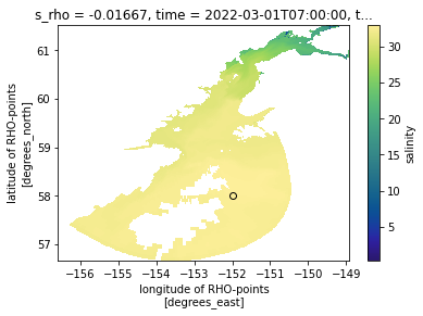
da1 = ds1['salt']
lon0, lat0 = -152, 58
lons, lats = [-151, -152], [59,58]
2D lon/lat
1 lon/lat pair
%%time
output = da1.em.interp2d(lon0, lat0)
output
CPU times: user 8.95 s, sys: 2.08 s, total: 11 s
Wall time: 30.1 s
<xarray.DataArray 'salt' (time: 2, s_rho: 30)>
32.94 32.94 32.94 32.94 32.94 32.94 ... 32.87 32.87 32.87 32.87 32.87 32.87
Coordinates: (5)
Attributes: (8)
Surface value for first time matches map:
cmap=cmo.haline
mappable = da1.cf.isel(T=0, Z=-1).cf.plot(x='longitude', y='latitude', cmap=cmap)
vmin, vmax = mappable.get_clim()
plt.scatter(lon0, lat0, c=output.cf.isel(T=0, Z=-1).values, cmap=cmap, vmin=vmin, vmax=vmax, edgecolors='k')
<matplotlib.collections.PathCollection at 0x170c1bac0>
To retrieve the values:
output.values
output.values
array([[32.93971 , 32.939648, 32.939594, 32.93954 , 32.939472, 32.939392,
        32.939293, 32.93917 , 32.93898 , 32.93863 , 32.937885, 32.936424,
        32.933247, 32.92608 , 32.918026, 32.910328, 32.903812, 32.898037,
        32.892227, 32.88485 , 32.877373, 32.875435, 32.875843, 32.87596 ,
        32.875977, 32.875988, 32.875996, 32.875996, 32.87599 , 32.875977],
       [32.938396, 32.93832 , 32.938255, 32.93819 , 32.938118, 32.93803 ,
        32.93791 , 32.93775 , 32.937523, 32.937138, 32.9364  , 32.934933,
        32.931953, 32.92531 , 32.917496, 32.90954 , 32.90272 , 32.896683,
        32.89059 , 32.882954, 32.8751  , 32.87288 , 32.87316 , 32.873245,
        32.873253, 32.873257, 32.873257, 32.873253, 32.873245, 32.873226]],
      dtype=float32)
To retrieve the associated depths:
output.cf['vertical'].values
output.cf['vertical'].values
array([-0.98333333, -0.95      , -0.91666667, -0.88333333, -0.85      ,
       -0.81666667, -0.78333333, -0.75      , -0.71666667, -0.68333333,
       -0.65      , -0.61666667, -0.58333333, -0.55      , -0.51666667,
       -0.48333333, -0.45      , -0.41666667, -0.38333333, -0.35      ,
       -0.31666667, -0.28333333, -0.25      , -0.21666667, -0.18333333,
       -0.15      , -0.11666667, -0.08333333, -0.05      , -0.01666667])
multiple lon/lat pairs
%%time
da1.em.interp2d(lons, lats)
CPU times: user 8.4 s, sys: 1.72 s, total: 10.1 s
Wall time: 27.6 s
<xarray.DataArray 'salt' (time: 2, s_rho: 30, lat: 2, lon: 2)>
32.49 32.05 32.95 32.94 32.49 32.05 ... 32.78 32.87 31.97 32.03 32.78 32.87
Coordinates: (5)
Attributes: (8)
3D: lon, lat, iZ
Return model output interpolated to lon, lat, Z value.
da1.em.interp2d(lon0, lat0, Z=-40)
<xarray.DataArray 'salt' (time: 2)>
nan nan
Coordinates: (5)
Attributes: (8)
Return model output interpolated to lon, lat, at index iZ in Z dimension.
da1.em.interp2d(lon0, lat0, iZ=-1)
<xarray.DataArray 'salt' (time: 2)>
32.88 32.87
Coordinates: (5)
Attributes: (8)
Note that it is not currently possible to interpolate in depth when there are both multiple times and locations.
If uncommented, the following cell will return:
NotImplementedError: Currently it is not possible to interpolate in depth with more than 1 other (time) dimension.
# da1.em.interp2d(lons, lats, Z=-40)